Object Detection using SSD Mobilenet V2
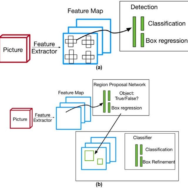
Object detection is a computer vision technology related to image processing that deals with detecting instances of semantic objects of a certain class in digital images and videos. With the advent of deep neural networks, object detection has taken the center stage in the development of computer vision with many models developed such as R-CNN (Regional Convolutional Neural Network) and it's variant (Faster-RCNN), Single Shot Detectors (SSD) models as well as the famous You Only Look Once (YOLO) models and it’s many versions. Typically object detection models are categorized into two major architectural types: one (single) stage object detectors such as YOLO and SSD and two (dual) stage object detectors such as R-CNN. The major difference between the two is that in the two-stage object detection models, the region of interest is first determined and the detection is then performed only on the region of interest. This implies that the two-stage object detection models are generally more accurate than the one-stage ones but require more computational resources and are slower. The below figure shows a representation of the two types of object detection models with (a) being one-stage detection and (b) being a two-stage detection model.

SSD Mobilenet V2 is a one-stage object detection model which has gained popularity for its lean network and novel depthwise separable convolutions. It is a model commonly deployed on low compute devices such as mobile (hence the name Mobilenet) with high accuracy performance. Today, we will be working through the entire process of training a custom image or a dataset using the SSD-Mobilenet V2 architecture. Just to give you a sneak peek of the outcome, below will be the result of training the SSD architecture for the detection of a tree. The entire training process will take place on the Colab which has GPU capabilities for faster training. The reason why I selected a tree for object detection is that the tree is not available in any of the existing coco-dataset and therefore the image pipeline for the tree needs to be built from scratch.

Data Acquisition & Image Tagging
The journey of training an object detection model begins with data acquisition. Although there exist many ways of automating the process, in this specific training case, data acquisition was done manually to filter out noisy images and to ensure the quality of the training dataset. Once the data is acquired, the images in the dataset need to be tagged. Image tagging was completed using the LabelImg software, which is an open-source python-based implementation of a system that tags the bounding boxes and records them in an XML file. Below is an image taken during the tagging of the pictures.

The generated result of the image tagging efforts is an XML file that encompasses the bounding boxes of the tagged images. A sample XML file is shown below for reference:

Preparing dataset
With the image acquisition and tagging done, you will be happy to know that most of the manual work is now completed. The output generated from the tagged image dataset is an XML file containing the bounding box coordinates of the hand-tagged images. However, neural net models cannot parse XML files and require a specific format called Tensor Records. Hence the next set of code involves the conversion of the XML file to an intermediate CSV output and then the final conversion of the CSV output to TF-Records.
The CSV file output for both the train and validation dataset is then converted to TF-Records format using the below code. There are several things to take note of over here. While creating the TF-Records file, the label map needs to be generated. The label map is essentially an encoder for the classes to be trained as the neural net predicts only in numbers after the final sigmoid layer. In our case, since we are only training for trees, there is only a single label “1” required for trees.
With the TF record files generated, the next stage involves the creation of the object detection text file. The object detection text file will be referred to by the model to determine the text on the bounding box and needs to correspond to the item label. For the tree detection problem statement, the object detection text file is shown below:
item {id: 1
name: 'tree'}
With this, the data preparing stage is complete in the model building.
Configuring Training
Configuration of the training involves the selection of the model as well as model parameters such as batch size, number of steps, training, and testing TF-Records directory. Thankfully, TensorFlow’s object detection pipeline comes with a pre-configured file that optimizes most of the configuration selection for efficient model training. We can download this configuration file by using the below command.
If we take a look at the configuration file, there are several parameters that are required to be updated. Firstly, we need to configure the path to the label map or the object detection text file that we created earlier so that the model is aware of the label to place on the image once detected. Next, we need to provide the path to the training and testing TF-Records files. The number of classes is set as 1 and a default batch size of 16 was set for the training. The number of training steps, which refers simply to the number of training epochs is then set to 1000. The SSD Mobilenet V2 model is then downloaded and the location to the checkpoint file is also incorporated in the config file. The below code provides an effective way to make these changes within Colab instead of manually typing them.
With this training configuration file built, we proceed to the more fun part — training the model 😃
Training, Monitoring, and testing
To simply start training the model, run the below code which will initiate the training pipeline in TensorFlow. Remember to provide the logging parameter so that the results of the model training can be observed in the tensorboard.

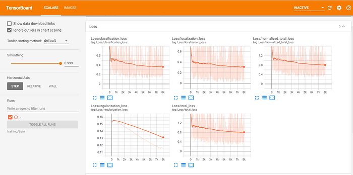
The results shown above depict the training over 8000 steps or epochs with a batch size of 16. As observed, the loss profiles have tapered down as the model has extracted the key features and learned the representation of a tree. With the training completed, the model is saved to the directory and can be used for testing on new sets of images.
To improve the variance and also test the batch normalization capability of the SSD-Mobilenet V2, I chose a diverse range of pictures including some black and white to check if the model is able to detect the trees. In order to test the model, the following code can be run which includes loading the newly trained model.
Next, with the model loaded, the inference can be performed by running the following code on all the test images.

And Viola! you have it, the model is able to successfully infer the trees present in the picture and performs quite well at it too. This concludes the development of object detection and inference pipeline for custom objects.
Conclusion
In this article, we went through the entire journey of training an object detection model for a customized dataset starting from data acquisition to image data tagging to finally training and validating the model. The model chosen was a one-stage object detection model (SSD Mobilenet V2) which can be used for many low compute and mobile devices. Although for simplicity we went through the training and validation for a single object, this training pipeline is scalable and can be applied for multiple objects in the customized dataset. So with that, happy training 😃
The Colab resource used for the object detection training is saved in the following repository: https://github.com/vid1994/ObjectDetection and the image dataset can be accessed https://drive.google.com/drive/folders/18BKO9f-Z-y-3SAw8BZhJrmXUX4vMKEUJ?usp=sharing
References
https://machinelearningmastery.com/object-recognition-with-deep-learning/